---
title: "Organising Large Projects with Sub-Pipelines"
output: rmarkdown::html_vignette
vignette: >
  %\VignetteIndexEntry{sub-pipelines}
  %\VignetteEngine{knitr::rmarkdown}
  %\VignetteEncoding{UTF-8}
---

```{r setup, include = FALSE}
knitr::opts_chunk$set(
  collapse = TRUE,
  comment = "#>"
)
```

This vignette introduces `rxp_pipeline()`, a function for organising large
projects into logical sub-pipelines. This feature is particularly useful when
working on complex projects with multiple phases (e.g., ETL, Modelling, Reporting)
or when collaborating in teams where different members work on different parts
of the pipeline.

## Large Pipelines Become Unwieldy

As pipelines grow, a single `gen-pipeline.R` file can become difficult to
manage. Consider a data science project with:
- Data extraction and cleaning (ETL)
- Feature engineering
- Model training
- Model evaluation
- Report generation

Putting all derivations in one file makes it hard to:

- Navigate the code
- Understand which derivations belong to which phase
- Collaborate across team members
- Reuse pipeline components in other projects

To solve this issue, you can define your project using sub-pipelines and join
them into a master pipeline using `rxp_pipeline()`.

This allows you to:

1. **Organise** derivations into named groups
2. **Colour-code** groups for visual distinction in DAG visualisations
3. **Modularise** your code across multiple R scripts

### Basic Usage

A project with sub-pipelines would look something like this:


```
my-project/
├── default.nix           # Nix environment (generated by rix)
├── gen-env.R             # Script to generate default.nix
├── gen-pipeline.R        # MASTER SCRIPT: combines all sub-pipelines
└── pipelines/
    ├── 01_data_prep.R    # Data preparation sub-pipeline
    ├── 02_analysis.R     # Analysis sub-pipeline
    └── 03_reporting.R    # Reporting sub-pipeline
```

Each sub-pipeline file returns a list of derivations:

```{r sub-pipeline-1, eval = FALSE}
# Data Preparation Sub-Pipeline
# pipelines/01_data_prep.R
library(rixpress)

list(
  rxp_r(name = raw_mtcars, expr = mtcars),
  rxp_r(name = clean_mtcars, expr = dplyr::filter(raw_mtcars, am == 1)),
  rxp_r(name = selected_mtcars, expr = dplyr::select(clean_mtcars, mpg, cyl, hp, wt))
)
```

The `rxp_pipeline()` function takes:

- **name**: A descriptive name for this group of derivations
- **path**: Either a **file path** to an R script returning a list of derivations (recommended), or a list of derivation objects.
- **color**: Optional CSS color name or hex code for DAG visualisation

The second sub-pipeline:

```{r sub-pipeline-2, eval = FALSE}
# Analysis Sub-Pipeline
# pipelines/02_analysis.R
library(rixpress)

list(
  rxp_r(name = summary_stats, expr = summary(selected_mtcars)),
  rxp_r(name = mpg_model, expr = lm(mpg ~ hp + wt, data = selected_mtcars)),
  rxp_r(name = model_coefs, expr = coef(mpg_model))
)
```

The master script becomes very clean, as `rxp_pipeline` handles sourcing the files:

```{r master-script, eval = FALSE}
# gen-pipeline.R
library(rixpress)

# Create named pipelines with colours by pointing to the files
pipe_data_prep <- rxp_pipeline(
  name = "Data Preparation",
  path = "pipelines/01_data_prep.R",
  color = "#E69F00"
)

pipe_analysis <- rxp_pipeline(
  name = "Statistical Analysis",
  path = "pipelines/02_analysis.R",
  color = "#56B4E9"
)

# Build combined pipeline
rxp_populate(list(pipe_data_prep, pipe_analysis), project_path = ".", build = TRUE)
```

## Visualising Sub-Pipelines

When sub-pipelines are defined, visualisation tools use pipeline colours:

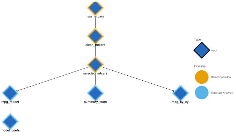
1. **Interactive Network** (`rxp_visnetwork()`) and **Static DAG** (`rxp_ggdag()`) both use a dual-encoding approach:
   - **Node fill (interior)**: Derivation type colour (R = blue, Python = yellow, etc.)
   - **Node border (thick stroke)**: Pipeline group colour
   This allows you to see both what *type* of computation each node is and which *pipeline* it belongs to.

<figure>
<img src="https://raw.githubusercontent.com/ropensci/rixpress/refs/heads/main/vignettes/subpipelines.png" alt="Subpipelines are coloured." />
<figcaption aria-hidden="true">
Subpipelines are coloured.
</figcaption>
</figure>

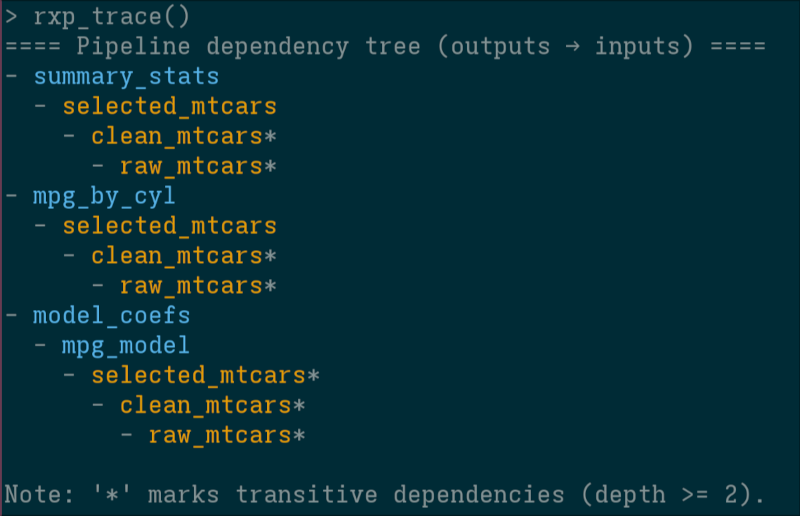
3. **Trace**: `rxp_trace()` output in the console is coloured by pipeline (using the `cli` package).

<figure>
<img src="https://raw.githubusercontent.com/ropensci/rixpress/refs/heads/main/vignettes/subpipelines_trace.png" alt="If your terminal supports it, derivation names are coloured according to the chosen sub-pipeline colour." />
<figcaption aria-hidden="true">
If your terminal supports it, derivation names are coloured according to the chosen sub-pipeline colour.
</figcaption>
</figure>

### Switching Between Colour Modes

```{r color-modes, eval = FALSE}
# Dual encoding: fill = type, border = pipeline (default when pipelines are defined)
rxp_ggdag(color_by = "pipeline")

# Colour entirely by derivation type (rxp_r, rxp_py, etc.) - original behaviour
rxp_ggdag(color_by = "type")
```

## How It Works Internally

When you call `rxp_populate()` with `rxp_pipeline` objects:

1. **Flattening**: Pipelines are flattened to a single list of derivations
2. **Metadata Preservation**: Each derivation retains `pipeline_group` and `pipeline_color`
3. **DAG Generation**: `dag.json` includes pipeline metadata
4. **Visualisation**: `rxp_visnetwork()` and `rxp_ggdag()` read this metadata

## Best Practices

1. **Use descriptive pipeline names**: "Data Preparation" is better than "ETL"
2. **Choose contrasting colours**: Use [ColorBrewer](https://colorbrewer2.org/) palettes
3. **Keep sub-pipelines focused**: One logical phase per sub-pipeline
4. **Order your files**: Use numeric prefixes (01_, 02_, etc.)

## Conclusion

`rxp_pipeline()` provides a simple yet powerful way to organise complex
pipelines. By grouping derivations into logical units, you can:

- Keep your code organised and maintainable
- Enable team collaboration on different parts of the pipeline
- Visualise the structure of your workflow with meaningful colours
- Reuse sub-pipelines across projects

For a working example, see the `subpipelines` demo in the
[rixpress_demos](https://github.com/b-rodrigues/rixpress_demos) repository.