
Describe and understand your model’s parameters!
parameters’ primary goal is to provide utilities for processing the parameters of various statistical models (see here for a list of supported models). Beyond computing p-values, CIs, Bayesian indices and other measures for a wide variety of models, this package implements features like bootstrapping of parameters and models, feature reduction (feature extraction and variable selection), or tools for data reduction like functions to perform cluster, factor or principal component analysis.
Another important goal of the parameters package is to facilitate and streamline the process of reporting results of statistical models, which includes the easy and intuitive calculation of standardized estimates or robust standard errors and p-values. parameters therefor offers a simple and unified syntax to process a large variety of (model) objects from many different packages.
![]()
| Type | Source | Command |
|---|---|---|
| Release | CRAN | install.packages("parameters") |
| Development | r - universe | install.packages("parameters", repos = "https://easystats.r-universe.dev") |
| Development | GitHub | remotes::install_github("easystats/parameters") |
Tip
Instead of
library(parameters), uselibrary(easystats). This will make all features of the easystats-ecosystem available.To stay updated, use
easystats::install_latest().
![]()
![]()
![]()
Click on the buttons above to access the package documentation and the easystats blog, and check-out these vignettes:
In case you want to file an issue or contribute in another way to the package, please follow this guide. For questions about the functionality, you may either contact us via email or also file an issue.
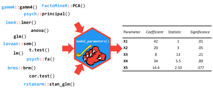
The model_parameters()
function (that can be accessed via the parameters()
shortcut) allows you to extract the parameters and their characteristics
from various models in a consistent way. It can be considered as a
lightweight alternative to broom::tidy(),
with some notable differences:
standardize_names()).model <- lm(Sepal.Width ~ Petal.Length * Species + Petal.Width, data = iris)
# regular model parameters
model_parameters(model)
#> Parameter | Coefficient | SE | 95% CI | t(143) | p
#> -------------------------------------------------------------------------------------------
#> (Intercept) | 2.89 | 0.36 | [ 2.18, 3.60] | 8.01 | < .001
#> Petal Length | 0.26 | 0.25 | [-0.22, 0.75] | 1.07 | 0.287
#> Species [versicolor] | -1.66 | 0.53 | [-2.71, -0.62] | -3.14 | 0.002
#> Species [virginica] | -1.92 | 0.59 | [-3.08, -0.76] | -3.28 | 0.001
#> Petal Width | 0.62 | 0.14 | [ 0.34, 0.89] | 4.41 | < .001
#> Petal Length × Species [versicolor] | -0.09 | 0.26 | [-0.61, 0.42] | -0.36 | 0.721
#> Petal Length × Species [virginica] | -0.13 | 0.26 | [-0.64, 0.38] | -0.50 | 0.618
# standardized parameters
model_parameters(model, standardize = "refit")
#> Parameter | Coefficient | SE | 95% CI | t(143) | p
#> -------------------------------------------------------------------------------------------
#> (Intercept) | 3.59 | 1.30 | [ 1.01, 6.17] | 2.75 | 0.007
#> Petal Length | 1.07 | 1.00 | [-0.91, 3.04] | 1.07 | 0.287
#> Species [versicolor] | -4.62 | 1.31 | [-7.21, -2.03] | -3.53 | < .001
#> Species [virginica] | -5.51 | 1.38 | [-8.23, -2.79] | -4.00 | < .001
#> Petal Width | 1.08 | 0.24 | [ 0.59, 1.56] | 4.41 | < .001
#> Petal Length × Species [versicolor] | -0.38 | 1.06 | [-2.48, 1.72] | -0.36 | 0.721
#> Petal Length × Species [virginica] | -0.52 | 1.04 | [-2.58, 1.54] | -0.50 | 0.618
# heteroscedasticity-consitent SE and CI
model_parameters(model, vcov = "HC3")
#> Parameter | Coefficient | SE | 95% CI | t(143) | p
#> -------------------------------------------------------------------------------------------
#> (Intercept) | 2.89 | 0.43 | [ 2.03, 3.75] | 6.66 | < .001
#> Petal Length | 0.26 | 0.29 | [-0.30, 0.83] | 0.92 | 0.357
#> Species [versicolor] | -1.66 | 0.53 | [-2.70, -0.62] | -3.16 | 0.002
#> Species [virginica] | -1.92 | 0.77 | [-3.43, -0.41] | -2.51 | 0.013
#> Petal Width | 0.62 | 0.12 | [ 0.38, 0.85] | 5.23 | < .001
#> Petal Length × Species [versicolor] | -0.09 | 0.29 | [-0.67, 0.48] | -0.32 | 0.748
#> Petal Length × Species [virginica] | -0.13 | 0.31 | [-0.73, 0.48] | -0.42 | 0.675library(lme4)
model <- lmer(Sepal.Width ~ Petal.Length + (1 | Species), data = iris)
# model parameters with CI, df and p-values based on Wald approximation
model_parameters(model)
#> # Fixed Effects
#>
#> Parameter | Coefficient | SE | 95% CI | t(146) | p
#> ------------------------------------------------------------------
#> (Intercept) | 2.00 | 0.56 | [0.89, 3.11] | 3.56 | < .001
#> Petal Length | 0.28 | 0.06 | [0.16, 0.40] | 4.75 | < .001
#>
#> # Random Effects
#>
#> Parameter | Coefficient | SE | 95% CI
#> -----------------------------------------------------------
#> SD (Intercept: Species) | 0.89 | 0.46 | [0.33, 2.43]
#> SD (Residual) | 0.32 | 0.02 | [0.28, 0.35]
# model parameters with CI, df and p-values based on Kenward-Roger approximation
model_parameters(model, ci_method = "kenward", effects = "fixed")
#> # Fixed Effects
#>
#> Parameter | Coefficient | SE | 95% CI | t | df | p
#> -------------------------------------------------------------------------
#> (Intercept) | 2.00 | 0.57 | [0.07, 3.93] | 3.53 | 2.67 | 0.046
#> Petal Length | 0.28 | 0.06 | [0.16, 0.40] | 4.58 | 140.98 | < .001Besides many types of regression models and packages, it also works for other types of models, such as structural models (EFA, CFA, SEM…).
library(psych)

model <- psych::fa(attitude, nfactors = 3)
model_parameters(model)
#> # Rotated loadings from Factor Analysis (oblimin-rotation)
#>
#> Variable   |   MR1 |   MR2 |   MR3 | Complexity | Uniqueness
#> ------------------------------------------------------------
#> rating     |  0.90 | -0.07 | -0.05 |       1.02 |       0.23
#> complaints |  0.97 | -0.06 |  0.04 |       1.01 |       0.10
#> privileges |  0.44 |  0.25 | -0.05 |       1.64 |       0.65
#> learning   |  0.47 |  0.54 | -0.28 |       2.51 |       0.24
#> raises     |  0.55 |  0.43 |  0.25 |       2.35 |       0.23
#> critical   |  0.16 |  0.17 |  0.48 |       1.46 |       0.67
#> advance    | -0.11 |  0.91 |  0.07 |       1.04 |       0.22
#>
#> The 3 latent factors (oblimin rotation) accounted for 66.60% of the total variance of the original data (MR1 = 38.19%, MR2 = 22.69%, MR3 = 5.72%).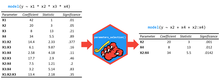
select_parameters()
can help you quickly select and retain the most relevant predictors
using methods tailored for the model type.
lm(disp ~ ., data = mtcars) |>
  select_parameters() |>
  model_parameters()
#> Parameter   | Coefficient |     SE |            95% CI | t(26) |      p
#> -----------------------------------------------------------------------
#> (Intercept) |      141.70 | 125.67 | [-116.62, 400.02] |  1.13 | 0.270
#> cyl         |       13.14 |   7.90 | [  -3.10,  29.38] |  1.66 | 0.108
#> hp          |        0.63 |   0.20 | [   0.22,   1.03] |  3.18 | 0.004
#> wt          |       80.45 |  12.22 | [  55.33, 105.57] |  6.58 | < .001
#> qsec        |      -14.68 |   6.14 | [ -27.31,  -2.05] | -2.39 | 0.024
#> carb | -28.75 | 5.60 | [ -40.28, -17.23] | -5.13 | < .001There is no standardized approach to drawing conclusions based on the available data and statistical models. A frequently chosen but also much criticized approach is to evaluate results based on their statistical significance (Amrhein, Korner-Nievergelt, & Roth, 2017).
A more sophisticated way would be to test whether estimated effects exceed the “smallest effect size of interest”, to avoid even the smallest effects being considered relevant simply because they are statistically significant, but clinically or practically irrelevant (Lakens, 2024; Lakens, Scheel, & Isager, 2018). A rather unconventional approach, which is nevertheless advocated by various authors, is to interpret results from classical regression models in terms of probabilities, similar to the usual approach in Bayesian statistics (Greenland, Rafi, Matthews, & Higgs, 2022; Rafi & Greenland, 2020; Schweder, 2018; Schweder & Hjort, 2003; Vos & Holbert, 2022).
The parameters package provides several options or functions to aid statistical inference. These are, for example:
equivalence_test(),
to compute the (conditional) equivalence test for frequentist
modelsp_significance(),
to compute the probability of practical significance, which can
be conceptualized as a unidirectional equivalence testp_function(),
or consonance function, to compute p-values and compatibility
(confidence) intervals for statistical modelspd argument (setting pd = TRUE) in
model_parameters() includes a column with the
probability of direction, i.e. the probability that a parameter
is strictly positive or negative. See bayestestR::p_direction()
for details.s_value argument (setting
s_value = TRUE) in model_parameters() replaces
the p-values with their related S-values (@ Rafi &
Greenland, 2020)bootstrap = TRUE) or simulating draws from model
coefficients using simulate_model().
These samples can then be treated as “posterior samples” and used in
many functions from the bayestestR package.Most of the above shown options or functions derive from methods
originally implemented for Bayesian models (Makowski, Ben-Shachar, Chen,
& Lüdecke, 2019). However, assuming that model assumptions are met
(which means, the model fits well to the data, the correct model is
chosen that reflects the data generating process (distributional model
family) etc.), it seems appropriate to interpret results from classical
frequentist models in a “Bayesian way” (more details: documentation in
p_function()).
In order to cite this package, please use the following command:
citation("parameters")
To cite package 'parameters' in publications use:

  Lüdecke D, Ben-Shachar M, Patil I, Makowski D (2020). "Extracting,
  Computing and Exploring the Parameters of Statistical Models using
  R." _Journal of Open Source Software_, *5*(53), 2445.
  doi:10.21105/joss.02445 <https://doi.org/10.21105/joss.02445>.

A BibTeX entry for LaTeX users is

  @Article{,
    title = {Extracting, Computing and Exploring the Parameters of Statistical Models using {R}.},
    volume = {5},
    doi = {10.21105/joss.02445},
    number = {53},
    journal = {Journal of Open Source Software},
    author = {Daniel Lüdecke and Mattan S. Ben-Shachar and Indrajeet Patil and Dominique Makowski},
    year = {2020},
    pages = {2445},
}Please note that the parameters project is released with a Contributor Code of Conduct. By contributing to this project, you agree to abide by its terms.