![]()
![]()
The “MCT” in musicMCT stands for Modal Color Theory, a theory of musical scale structure developed by Paul Sherrill, “Modal Color Theory,” Journal of Music Theory 69/1 (2025): 1-49. The goal of this package is to give musicians and music scholars computational tools that make it easier to work with this theory. In a nutshell, Modal Color Theory models musical scales as points in a geometry. The locations of those points relative to various hyperplane arrangements tell us a lot about the scales’ internal structures and mutual relationships. The shape of those hyperplane arrangements gets pretty complex: for the important case of seven-note scales, the main arrangement has 42 hyperplanes in a 6-dimensional space. Computational tools are therefore very helpful.
If you’ve ever wondered why a piece of music uses one scale rather than another; if you want to know more about the jazz chord-scale concept of lydian being “bright” and locrian being “dark”; if you’ve ever wanted to design your own microtonal scale from scratch; if you’re a theorist who wants a geometrical perspective on concepts like voice leading and maximal evenness; if you’re an ethnomusicologist looking to interpret tuning data: musicMCT might be useful to you.
You can install the latest released version of musicMCT from CRAN with:
install.packages("musicMCT")Alternatively, you can install the development version of musicMCT from GitHub with:
install.packages("remotes")
remotes::install_github("satbq/musicMCT")
In addition to the package itself, you will probably want to use the following large files which contain data about the MCT geometries:
Download these files, save them to your working directory, and load them with:
representative_scales <- readRDS("representative_scales.rds")
representative_signvectors <- readRDS("representative_signvectords.rds")
color_adjacencies <- readRDS("color_adjacencies.rds")For a detailed introduction to using this package, please see the introductory vignette.
As a very quick example, let’s define the most common “just intonation” version of the major scale and run a few tests on it:
library(musicMCT)
just_dia_frequency_ratios <- c(1, 9/8, 5/4, 4/3, 3/2, 5/3, 15/8)
just_dia <- 12 * log2(just_dia_frequency_ratios)

# This definition of the just diatonic explicitly derives it from the
# frequency ratios, which I've done to model that process for you. However,
# musicMCT also has a convenience function that will give us the
# same result much faster: try out j(dia) or j(1,2,3,4,5,6,7) for yourself.

# The modes of the scale are displayed as the columns in this matrix:
sim(just_dia)
#>           [,1]     [,2]      [,3]      [,4]     [,5]      [,6]     [,7]
#> [1,]  0.000000 0.000000  0.000000  0.000000 0.000000  0.000000 0.000000
#> [2,]  2.039100 1.824037  1.117313  2.039100 1.824037  2.039100 1.117313
#> [3,]  3.863137 2.941350  3.156413  3.863137 3.863137  3.156413 3.156413
#> [4,]  4.980450 4.980450  4.980450  5.902237 4.980450  5.195513 4.980450
#> [5,]  7.019550 6.804487  7.019550  7.019550 7.019550  7.019550 6.097763
#> [6,]  8.843587 8.843587  8.136863  9.058650 8.843587  8.136863 8.136863
#> [7,] 10.882687 9.960900 10.175963 10.882687 9.960900 10.175963 9.960900

# A few pieces of evidence that the scale is "pairwise well-formed":
asword(just_dia)
#> [1] 3 2 1 3 2 3 1
howfree(just_dia)
#> [1] 2
isgwf(just_dia)
#> [1] TRUE

# A 15 equal-tempered approximation of just-dia which preserves its "color":
quantized_just_dia <- quantize_color(just_dia)
print(quantized_just_dia)
#> $set
#> [1]  0  3  5  6  9 11 14
#>
#> $edo
#> [1] 15

# Finally, let's see a rough brightness graph for the scale. (R can assemble the
# necessary information, but musicMCT doesn't yet make the graphs pretty.)
brightnessgraph(quantized_just_dia$set, edo=quantized_just_dia$edo)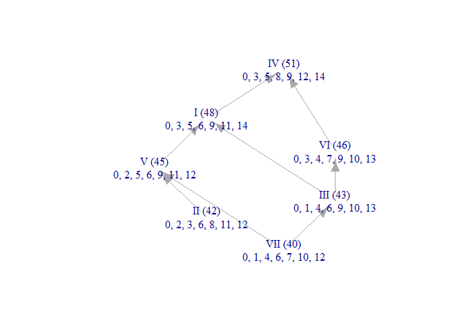
Thanks to Nate Mitchell for designing the package’s hex sticker logo.