ggcircular

ggcircular is a ggplot2 extension for circular, axial and directional data. It provides layers, scales, coordinate helpers, summaries and diagnostics for angles measured on a periodic scale.

The package is designed for exploratory graphics, teaching examples and reproducible statistical workflows involving directions, bearings, orientations, times of day, turn angles and other circular measurements.

Installation

Not on CRAN yet

ggcircular is not on CRAN yet. Install it from GitHub while the API is being stabilized for a first CRAN submission.

Install the development release from GitHub:

install.packages("remotes")
remotes::install_github("AurelienNicosiaULaval/ggcircular")

Or clone with SSH and install locally:

git clone git@github.com:AurelienNicosiaULaval/ggcircular.git
cd ggcircular
R -q -e 'devtools::install(upgrade = "never")'

Quick Start

library(ggplot2)
library(dplyr)
library(ggcircular)

wind_directions |>
  filter(season == "winter") |>
  ggplot(aes(x = direction)) +
  geom_rose(aes(y = after_stat(density), fill = after_stat(density)), bins = 24, alpha = 0.78) +
  geom_circular_density(linewidth = 1.1, colour = "#123C4A") +
  geom_mean_direction(length = "resultant", colour = "#E4572E", linewidth = 1.1) +
  scale_x_circular_compass() +
  coord_circular(zero = "north", direction = "clockwise") +
  labs(fill = "density", title = "Winter wind directions") +
  theme_circular()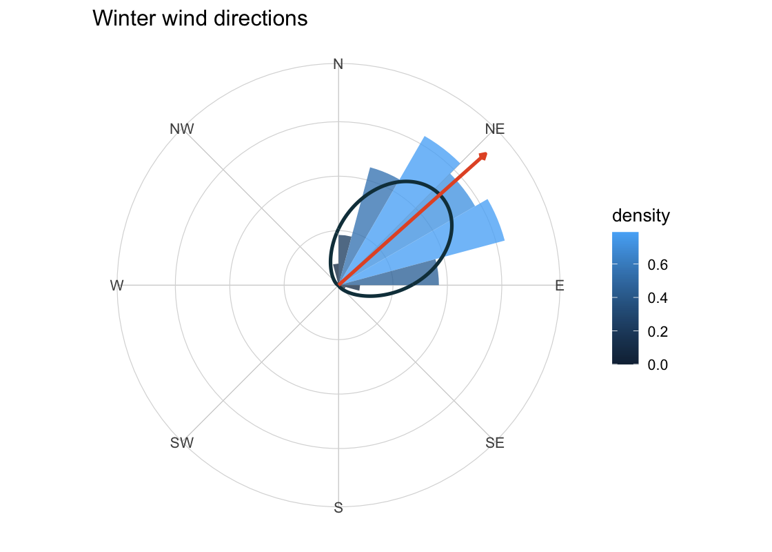

What It Does

Workflow	Main helpers
Rose diagrams and circular histograms	`geom_rose()`, `stat_rose()`
Circular density estimation	`geom_circular_density()`, `stat_circular_density()`
Mean direction and concentration	`geom_mean_direction()`, `circular_summary()`, `estimate_kappa()`
Circular confidence intervals and tests	`circular_mean_ci()`, `rayleigh_test()`, `watson_williams_test()`, `stat_circular_test()`
Axial orientations modulo pi	`axial = TRUE` in summaries and layers
Theoretical circular distributions	`stat_vonmises()`, `stat_wrapped_normal()`, `stat_uniform_circular()`
Mixtures of von Mises components	`fit_vonmises_mixture()`, `stat_vonmises_mixture()`
Movement and state-angle graphics	`mutate_directional_features()`, `geom_direction_arrow()`, `plot_state_angles()`
Angular model diagnostics	`circular_residuals()`, `circular_model_diagnostics()`, `autoplot()` methods
Spherical and posterior helpers	`spherical_summary()`, `as_circular_draws()`, `summarise_circular_draws()`

Design Principles

Angles are stored and computed in radians.
Scales handle display labels in radians, degrees, hours or compass labels.
Directional data use period 2 * pi.
Axial data use period pi through axial = TRUE.
Heavy packages remain optional and are accessed with explicit availability checks.
Outputs are standard ggplot objects, tibbles or familiar test objects.

Conventions for Directions and Bearings

The default mathematical convention is zero = "east" with angles increasing counterclockwise. This matches the usual unit circle.

Compass bearings use zero = "north" with angles increasing clockwise. Use scale_x_circular_compass() together with coord_circular(zero = "north", direction = "clockwise") for bearing-like data such as wind direction or movement headings.

Axial data, such as unoriented lines, are different again: 0 and pi represent the same orientation. Use axial = TRUE in summaries and layers for these data.

Summaries

circular_summary() respects existing dplyr groups and returns mean direction, resultant length, circular variance, circular standard deviation and an estimated von Mises concentration parameter. estimate_kappa() is a descriptive piecewise approximation from the sample resultant length, not a full inferential fit.

wind_directions |>
  circular_summary(direction, season) |>
  mutate(
    mean_degrees = round(rad_to_deg(mean), 1),
    Rbar = round(Rbar, 3),
    kappa = round(kappa, 2)
  ) |>
  select(season, n, mean_degrees, Rbar, kappa)
#> # A tibble: 4 × 5
#>   season     n mean_degrees  Rbar kappa
#>   <chr>  <int>        <dbl> <dbl> <dbl>
#> 1 fall     131        310.  0.811  3
#> 2 spring   115        135.  0.802  2.89
#> 3 summer   138        223.  0.87   4.15
#> 4 winter   116         48.2 0.904  5.52

Axial Data

Axial observations identify opposite directions. For example, an orientation of 0 radians is equivalent to an orientation of pi radians. Use axial = TRUE to compute and display these data modulo pi.

ggplot(axial_orientations, aes(x = orientation, fill = group)) +
  geom_rose(bins = 18, axial = TRUE, alpha = 0.72) +
  geom_mean_direction(axial = TRUE, colour = "#123C4A", linewidth = 1) +
  scale_x_circular_degrees(limits = c(0, pi)) +
  coord_circular() +
  facet_wrap(~ group) +
  theme_circular()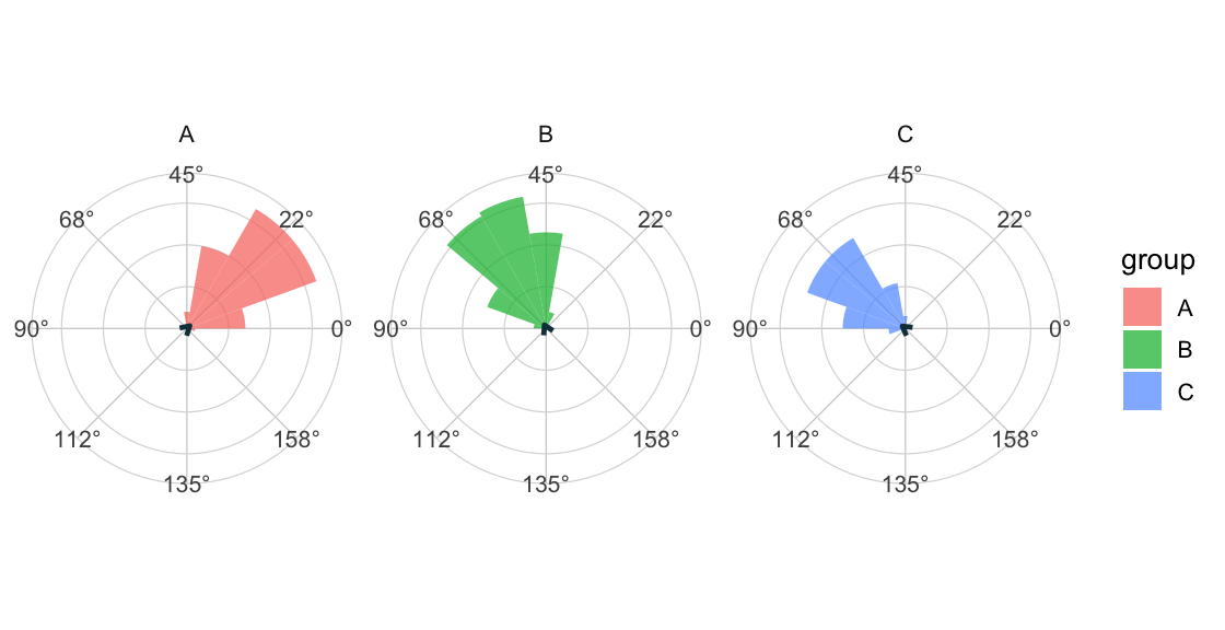

Directional Movement

ggcircular includes helpers for bearings, turn angles and state-specific angular distributions.

animal_steps |>
  filter(!is.na(turn_angle)) |>
  ggplot(aes(x = turn_angle, fill = state)) +
  geom_rose(bins = 24, alpha = 0.72) +
  geom_mean_direction(colour = "#123C4A", linewidth = 1) +
  scale_x_circular_degrees(
    breaks = deg_to_rad(c(0, 90, 180, 270)),
    labels = c("0", "90", "180", "270")
  ) +
  coord_circular() +
  facet_wrap(~ state) +
  theme_circular()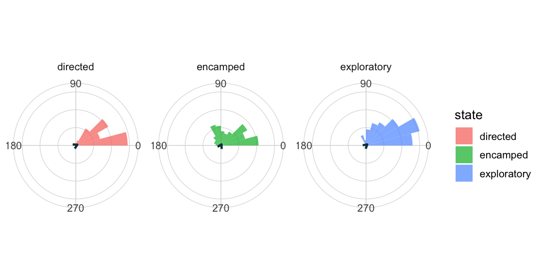

Mixtures of von Mises Distributions

Finite mixtures are fitted with an expectation-maximization routine and can be drawn directly on top of empirical rose diagrams. These fits are descriptive and depend on initialization, so use seed, nstart and diagnostic output when the mixture is substantively important.

set.seed(2026)

fit_mix <- fit_vonmises_mixture(
  wind_directions$direction,
  k = 2,
  init = "spaced",
  nstart = 3,
  seed = 2026
)

ggplot(wind_directions, aes(x = direction)) +
  geom_rose(aes(y = after_stat(density)), bins = 24, alpha = 0.42) +
  stat_vonmises_mixture(fit = fit_mix, linewidth = 1.2, colour = "#123C4A") +
  scale_x_circular_degrees() +
  coord_circular() +
  theme_circular()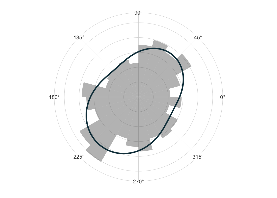

tidy_circular(fit_mix) |>
  mutate(
    mu_degrees = round(rad_to_deg(mu), 1),
    kappa = round(kappa, 2),
    proportion = round(proportion, 3)
  ) |>
  select(component, proportion, mu_degrees, kappa)
#> # A tibble: 2 × 4
#>   component proportion mu_degrees kappa
#>       <int>      <dbl>      <dbl> <dbl>
#> 1         1      0.328       51.6  1.45
#> 2         2      0.672      232.   0.77

Tests and Intervals

circular_mean_ci(
  wind_directions$direction,
  method = "bootstrap",
  R = 399,
  seed = 2026
) |>
  mutate(across(c(mean, lower, upper), rad_to_deg))
#> # A tibble: 1 × 7
#>    mean lower upper level method        n   Rbar
#>   <dbl> <dbl> <dbl> <dbl> <chr>     <int>  <dbl>
#> 1  235.  139.  354.  0.95 bootstrap   500 0.0494

rayleigh <- rayleigh_test(wind_directions$direction)

tibble::tibble(
  statistic = unname(rayleigh$statistic),
  n = unname(rayleigh$parameter),
  p_value = rayleigh$p.value,
  method = rayleigh$method
)
#> # A tibble: 1 × 4
#>   statistic     n p_value method
#>       <dbl> <int>   <dbl> <chr>
#> 1      1.22   500   0.295 Rayleigh test of circular uniformity

Optional Model Integrations

The package keeps heavier modeling ecosystems in Suggests. When available, these integrations add diagnostics without making them hard dependencies.

fit <- CircularRegression::consensus(direction ~ speed, data = wind_directions)

circular_model_diagnostics(fit)

autoplot(fit, type = "residuals_density")
autoplot(fit, type = "fitted_observed")

Optional helpers currently target:

CircularRegression-style angular, consensus and two-step objects through S3 class support.
momentuHMM state probabilities and Viterbi states.
posterior draw objects through posterior::as_draws_df().
circular tests when classical circular test implementations are available.

Experimental Features

The following pieces are intentionally available but still experimental:

angular model diagnostics for optional external model classes;
finite mixtures of von Mises distributions;
momentuHMM state-angle adapters;
spherical summaries and posterior draw helpers.

Experimental functions are documented and tested, but their return columns may still be refined before a CRAN release if validation reveals a better public contract.

Statistical Limitations

ggcircular is primarily a visualization and diagnostics package. It does not replace specialist inference workflows for circular statistics.

The automatic density bandwidth is a simple heuristic.
circular_mean_ci() is unreliable when the mean resultant length is close to zero because the mean direction is weakly identified.
rayleigh_test() is mainly sensitive to unimodal departures from uniformity.
watson_williams_test() relies on strong assumptions about group concentration and uses the optional circular implementation.
Multimodal data should usually be inspected with density or mixture graphics, not summarized only by one mean direction.

CRAN Readiness

The package is being prepared for a first CRAN submission. The release checklist currently includes:

R CMD check --as-cran on the final source tarball;
--run-donttest checks;
hard-dependency checks with _R_CHECK_FORCE_SUGGESTS_=false;
full-suggests checks when optional packages are available;
Linux R-devel, Linux R-release, macOS R-release and Windows R-release checks;
vignette build timing and source tarball size checks.

Longer articles are built for pkgdown and excluded from the CRAN tarball.

Vignettes

Start with:

vignette("ggcircular", package = "ggcircular")

Then see the pkgdown articles:

Contributing and Support

Contributions are welcome through focused GitHub issues and pull requests. See CONTRIBUTING.md, SUPPORT.md and CODE_OF_CONDUCT.md for contribution, support and conduct guidelines.

Development Status

ggcircular is currently experimental. The public API is usable, tested and documented, but may still evolve as more angular model classes and validation cases are added.

Current checks:

Local devtools::test() passes.
Local devtools::check(document = FALSE, args = "--as-cran", build_args = "--no-manual") is used before release commits.
GitHub Actions runs hard-dependency checks with _R_CHECK_FORCE_SUGGESTS_=false and full-suggests checks when optional packages are available.
GitHub Actions includes Linux R-devel plus Linux, macOS and Windows R-release.
pkgdown builds and publishes the website from main.

References

Fisher, N. I. (1993). Statistical Analysis of Circular Data. Cambridge University Press.
Jammalamadaka, S. R., and Sengupta, A. (2001). Topics in Circular Statistics. World Scientific.
Pewsey, A., Neuhäuser, M., and Ruxton, G. D. (2013). Circular Statistics in R. Oxford University Press.
Wickham, H. (2016). ggplot2: Elegant Graphics for Data Analysis. Springer.