![]()
The goal of edar is to provide some convenient functions to facilitate common tasks in exploratory data analysis.
Sou T (2025). edar: Convenient Functions for Exploratory Data Analysis. R package version 0.0.6, https://github.com/soutomas/edar.
# From CRAN - for the latest CRAN release
install.packages("edar")

# From GitHub - for the development version
# install.packages("pak")
pak::pak("soutomas/edar")It is often helpful to see a quick summary of the dataset.
library(edar)
#>
#> Attaching package: 'edar'
#> The following object is masked from 'package:stats':
#>
#>     filter

# Data
dat = mtcars |> mutate(across(c(am,carb,cyl,gear,vs),factor))

# Summaries of all continuous variables.
dat |> summ_by()
#> NB: Non-numeric variables are dropped.
#> Dropped: cyl vs am gear carb
#> Adding missing grouping variables: `name`
#> # A tibble: 6 × 10
#>   name      n   nNA   Mean      SD   Min    P25    Med    P75    Max
#>   <chr> <int> <int>  <dbl>   <dbl> <dbl>  <dbl>  <dbl>  <dbl>  <dbl>
#> 1 disp     32     0 231.   124.    71.1  121.   196.   326    472
#> 2 drat     32     0   3.60   0.535  2.76   3.08   3.70   3.92   4.93
#> 3 hp       32     0 147.    68.6   52     96.5  123    180    335
#> 4 mpg      32     0  20.1    6.03  10.4   15.4   19.2   22.8   33.9
#> 5 qsec     32     0  17.8    1.79  14.5   16.9   17.7   18.9   22.9
#> 6 wt       32     0   3.22   0.978  1.51   2.58   3.32   3.61   5.42

# Summaries of a selected variable after grouping.
dat |> summ_by(mpg,vs)
#> Adding missing grouping variables: `vs`
#> # A tibble: 2 × 10
#>   vs        n   nNA  Mean    SD   Min   P25   Med   P75   Max
#>   <fct> <int> <int> <dbl> <dbl> <dbl> <dbl> <dbl> <dbl> <dbl>
#> 1 0        18     0  16.6  3.86  10.4  14.8  15.6  19.1  26
#> 2 1        14     0  24.6  5.38  17.8  21.4  22.8  29.6  33.9

# Summaries of all categorical variables.
dat |> summ_cat()
#> NB: Numeric variables are dropped.
#> Dropped: mpg disp hp drat wt qsec
#> $cyl
#>    cyl  n percent
#>      4 11 0.34375
#>      6  7 0.21875
#>      8 14 0.43750
#>  Total 32 1.00000
#>
#> $vs
#>     vs  n percent
#>      0 18  0.5625
#>      1 14  0.4375
#>  Total 32  1.0000
#>
#> $am
#>     am  n percent
#>      0 19 0.59375
#>      1 13 0.40625
#>  Total 32 1.00000
#>
#> $gear
#>   gear  n percent
#>      3 15 0.46875
#>      4 12 0.37500
#>      5  5 0.15625
#>  Total 32 1.00000
#>
#> $carb
#>   carb  n percent
#>      1  7 0.21875
#>      2 10 0.31250
#>      3  3 0.09375
#>      4 10 0.31250
#>      6  1 0.03125
#>      8  1 0.03125
#> Total 32 1.00000Results can be viewed directly in a flextable object.
# Show data frame as a flextable object.
dat |> summ_by(mpg,vs) |> ft()
#> Adding missing grouping variables: `vs`
Variables can be quickly visualised for exploratory graphical analysis.
# Scatter plot showing correlation.
dat |> ggxy(hp,disp)
#> `geom_smooth()` using formula = 'y ~ x'
# Histograms of all continuous variables.
dat |> gghist()
#> NB: Non-numeric variables are dropped.
#> Dropped: cyl vs am gear carb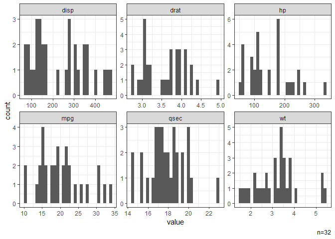
# Box plots stratified by categorical variables.
dat |> ggbox(mpg)
#> NB: Numeric variables are dropped.
#> Dropped: disp hp drat wt qsec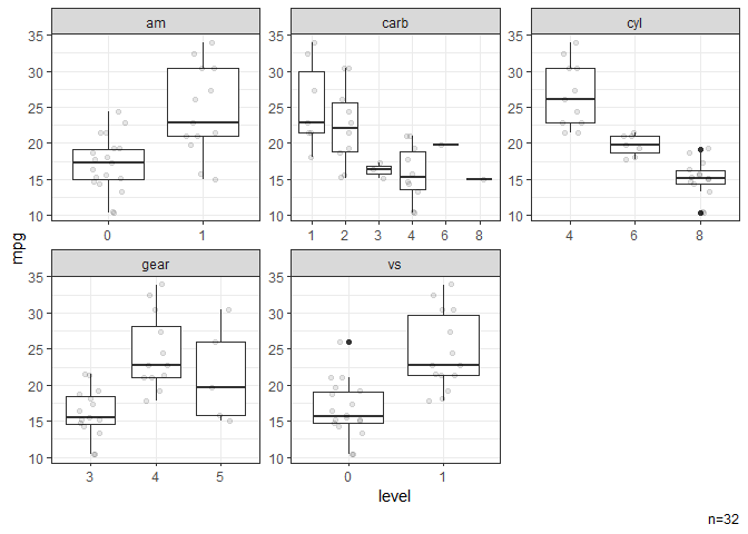
# Violin plots stratified by categorical variables.
dat |> ggvio(mpg)
#> NB: Numeric variables are dropped.
#> Dropped: disp hp drat wt qsec
#> Warning: Groups with fewer than two datapoints have been dropped.
#> ℹ Set `drop = FALSE` to consider such groups for position adjustment purposes.
#> Groups with fewer than two datapoints have been dropped.
#> ℹ Set `drop = FALSE` to consider such groups for position adjustment purposes.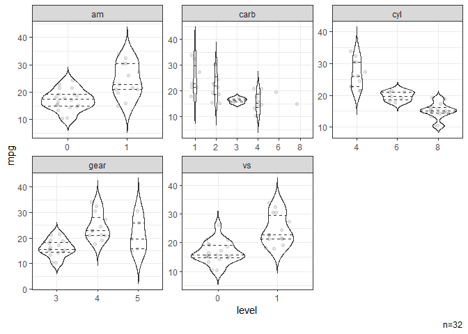
# Time-profile plot by subject.
Theoph |> ggtpp(Time, conc, id=Subject, xlab="Time [h]", ylab="Concentration [mg/L]")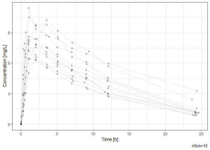
A label indicating the current source file with a time stamp can be easily generated for annotation.
# To generate a source file label for annotation.
lab = label_src()
# A source file label can be directly added to the flextable output.
dat |> summ_by(mpg,vs) |> ft(src=1)# A source file label can be directly added to a ggplot object.
p = dat |> ggxy(hp,disp)
p |> ggsrc()