

drugsens is a R-package that allows users to automatically analyze QuPath™’s output data from imaging analysis. Here we include a QuPath™ script (the same that we regularly use) to run reproducible QuPath™-based image analysis, and some examples on how drugsens can be used. For more detailed examples of QuPath™ scripting and usage please refer to QuPath™’s Documentation. This script should be placed into scripts manager within QuPath™. We tested this code with previous versions of QuPath™, but new versions should also be compatible. This package is complementary to the STAR protocol: Protocol for quantifying drug sensitivity in 3D patient-derived ovarian cancer models DOI: 10.1016/j.xpro.2024.103274.
Full documentation, function references, and step-by-step tutorials are available on the drugsens documentation site:
# Install from CRAN
install.packages("drugsens")

# Or install the latest development version from GitHub:
devtools::install_github("flalom/drugsens")
To install the development version from GitHub (optional),
devtools is used; if not installed yet, you can install it
with:
# Install devtools from CRAN
install.packages("devtools")

# Or the development version from GitHub:
# install.packages("pak")
pak::pak("r-lib/devtools")
You can have a look at devtools.
1. Cell Detection & Object Classification Script (STAR Protocol)
To add and run this script in the latest versions of QuPath (v0.4 / v0.5+):
Automate \(\rightarrow\)
Show script editor (or press Ctrl + [
on Windows/Linux, Cmd + [ on macOS).File \(\rightarrow\) New and
paste the Groovy script below (tip: you can also save it inside your
QuPath project’s scripts/ folder via
File \(\rightarrow\)
Save As... so it is always accessible under
Automate \(\rightarrow\)
Project scripts).<USER_DEFINED_PATH> and the
<...> metadata placeholders, and confirm that the
channel names (DAPI, E-Cadherin,
Cleaved Caspase 3) and single-measurement classifiers match
your project.Run
\(\rightarrow\)
Run (Ctrl + R /
Cmd + R). To process the entire project in batch, select
Run \(\rightarrow\)
Run for project in the Script Editor menu bar,
move your images to the Selected column, and click
OK.
/**
 * This QuPath script will take a full image as an annotation
 *
 * 1. Change path to export data, line 41
 * 2. Make sure that the channel order is DAPI, E-Cadherin, and Cleaved Caspase 3
 *      a) if this is not the case, change line 38 (setChannelNames) accordingly
 * 3. Your QuPath project must contain classifiers called "Cleaved Caspase 3" and "E-Cadherin"
 *    If you do not have them, you can download them from our repository,
 *    or create them yourself:
 *      i) In a image, create a selection of the full image (run lines 52-59)
 *      ii) Detect cells (run line 61)
 *      iii) In the Annotation tab, create new classification classes (Add class) called "Cleaved Caspase 3" and "E-Cadherin"
 *      iv) Create classifiers (from the menu Classify > Object Classification > Create single measurement classifier)
 *      v) Name the new classifier "Cleaved Caspase 3", and use following parameters
 *              Object filter = Detections (all)
 *              Channel filter = Cleaved Caspase 3
 *              Measurement = Nucleus: Cleaved Caspase 3 mean
 *              Threshold = 200 (value may differ for your image)
 *              Above threshold = Cleaved Caspase 3
 *      vi) Name the new classifier "E-Cadherin", and use following parameters
 *              Object filter = Detections (all)
 *              Channel filter = E-Cadherin
 *              Measurement = Nucleus: E-Cadherin mean
 *              Threshold = 180 (value may differ for your image)
 *              Above threshold = E-Cadherin
 * 4. Select Run -> Run for project
 *    It will go through all images in the project, run segmentation
 *    & apply those 2 classifiers we set up before.
 *
 * Note:
 *    You are encouraged to check and adjust the classifier before you run them on your own images.
 *    For this, follow steps 3.i) - 3.vi)
 */

import static qupath.lib.gui.scripting.QPEx.*

// Define the path for data export
def path = '<USER_DEFINED_PATH>'

setImageType('FLUORESCENCE');
setChannelNames ('DAPI', 'E-Cadherin', 'Cleaved Caspase 3')

def name = getProjectEntry().getImageName() + '.txt'
path = buildFilePath(path, '<PID>_<TISSUE>_<YYYY-MM-DD>_<SAMPLE_DOC>_<TREATMENT_INITIALS>_<CONCENTRATION>_<CONCENTRATION_UNITS>_<REPLICA_OR_NOT>_<TUMOR_MARKER>_<APOPTOTIC_MARKER>')
mkdirs(path)
path = buildFilePath(path, name)

// Create a new rectangle annotation & add it to the hierarchy
import qupath.lib.roi.RectangleROI
import qupath.lib.objects.PathAnnotationObject
def x_dim = getCurrentImageData().getServer().getWidth()
def y_dim = getCurrentImageData().getServer().getHeight()
def roi = new RectangleROI(0, 0, x_dim, y_dim)
def annotation = new PathAnnotationObject(roi)
addObject(annotation)
setSelectedObject(annotation)

runPlugin('qupath.imagej.detect.cells.WatershedCellDetection', '{"detectionImage": "DAPI",  "requestedPixelSizeMicrons": 0.5,  "backgroundRadiusMicrons": 8.0,  "medianRadiusMicrons": 0.0,  "sigmaMicrons": 2,  "minAreaMicrons": 5.0,  "maxAreaMicrons": 500.0,  "threshold": 45.0,  "watershedPostProcess": true,  "cellExpansionMicrons": 7.5,  "includeNuclei": true,  "smoothBoundaries": true,  "makeMeasurements": true}')
runObjectClassifier("Cleaved Caspase 3", "E-Cadherin")

saveAnnotationMeasurements(path)
print 'Results exported to ' + path
2. Measurement Export Script (Exporting to
.csv)
Once cell detection and classification have finished across your
project, use this second script to export the single-cell measurements
into the .csv format expected by drugsens:
In QuPath, go to Automate \(\rightarrow\)
Show script editor, then click
File \(\rightarrow\) New and
paste the script below (or click File \(\rightarrow\) Open...
to load the script_for_qupath.txt file generated in R by
generate_qupath_script()).
Set outputPath to your desired destination path and
filename following the <PID>_<TISSUE>_...
naming convention, and verify columnsToInclude (make sure
"Image" and "Name" are always
included).
In the Script Editor menu bar, click Run
\(\rightarrow\)
Run (Ctrl + R /
Cmd + R).
Note: Click
Run\(\rightarrow\)Run(notRun for project), becauseMeasurementExporterautomatically iterates through all images ingetProject().getImageList()and exports them in one step.
/**
 * QuPath script to export measurements from all analysed images in a project
 *
 * 1. Define columns you would like to export (line 28)
 * 2. In line 17, specify the path where to save your results
 */

import qupath.lib.gui.tools.MeasurementExporter
import qupath.lib.objects.PathCellObject
import qupath.lib.objects.PathDetectionObject
import qupath.lib.objects.PathAnnotationObject
import qupath.lib.objects.PathRootObject

// Choose your *full* output path
def outputPath = "<USER_DEFINED_PATH>/<PID>_<TISSUE>_<YYYY-MM-DD>_<SAMPLE_DOC>_<TREATMENT_INITIALS>_<CONCENTRATION>_<CONCENTRATION_UNITS>_<REPLICA_OR_NOT>_<TUMOR_MARKER>_<APOPTOTIC_MARKER>.csv"

// Get the list of all images in the current project
def project = getProject()
def imagesToExport = project.getImageList()

// Separate each measurement value in the output file with ","
def separator = ","

// Choose the columns that will be included in the export
// Note: if 'columnsToInclude' is empty, all columns will be included
def columnsToInclude = new String[]{"Image", "Name", "Class","Centroid X um","Centroid Y um","Nucleus: Area", "Nucleus: DAPI mean","Nucleus: E-Cadherin mean", "Nucleus: Cleaved caspase 3 mean", "Cell: Area","Cell: E-Cadherin mean", "Cell: Cleaved caspase 3 mean","Cytoplasm: E-Cadherin mean","Cytoplasm: Cleaved caspase 3 mean","Nucleus/Cell area ratio"}

// Choose the type of objects that the export will process
// Other possibilities include:
//    1. PathAnnotationObject
//    2. PathDetectionObject
//    3. PathRootObject
// Note: import statements should then be modified accordingly
def exportType = PathCellObject.class

def outputFile = new File(outputPath)

// Create the measurementExporter and start the export
def exporter  = new MeasurementExporter()
        .imageList(imagesToExport)            // Images from which measurements will be exported
        .separator(separator)                 // Character that separates values
        .includeOnlyColumns(columnsToInclude) // Columns are case-sensitive
        .exportType(exportType)               // Type of objects to export
        .exportMeasurements(outputFile)        // Start the export process

print "Done!"We recommend making a new project when working with
drugsens, to have clear and defined path. This will make
the data analysis much easier and reproducible. You can also set you
working directory with setwd().
To generate the QuPath export script
(script_for_qupath.txt) in tempdir() (or pass
output_dir = "." to save it in your working directory):
library("drugsens")
generate_qupath_script()
This function will generate a script_for_qupath.txt file
with the code that one can copy/paste into the QuPath’s script
manager. All the sections that contain <> should be
replaced with the user experimental information. The
columnsToInclude in the script should also be user defined,
depending on the markers used.
It is very important that the file naming structure of the QuPath’s
output is maintained for drugsens to work correctly.
Note: The
Imagecolumn must be present in the exported CSV fordrugsensto parse experimental metadata. For two-drug combinations, follow theCamelCaseconvention described under Bind QuPath files.
This command will generate a config_drugsens.txt file in
tempdir() (or in a custom project folder when
forcePath is supplied) that can be edited to map raw QuPath
marker names to clean names. In our case we replaced
"PathCellObject" with "onlyDAPIPositve".
make_run_config()Once config_drugsens.txt has been modified,
data_binding() loads it automatically into the package
configuration environment (pass forcePath if you stored
config_drugsens.txt in a project directory).
list_of_relabeling is a named list used to standardize raw
QuPath marker names without polluting .GlobalEnv. In case
the markers naming doesn’t need corrections/relabeling you can leave the
default configuration unchanged.
Note: We recommend concise, space-free
camelCasenames for cell markers inlist_of_relabeling:
- Start the marker name with a lowercase letter (for example,
onlyDAPIPositiveorcCASP3).- Avoid spaces or underscores between words.
- Capitalize the first letter of each subsequent word.
We present here a few mock datasets, as example workflow. Those files can be explored from the user’s R package path:
system.file("extdata/to_merge/", package = "drugsens")At first the data is a bunch of separate files which are difficult to make sense of; therefore as first step let’s bind them together into a single R dataframe! The example data can be bound together with this command:
bind_data <- data_binding(path_to_the_projects_folder = system.file("extdata/to_merge/", package = "drugsens"), files_extension_to_look_for = "csv")You will be now able to View(bind_data). You should see
all the image stacks from the QuPath in one dataframe. This dataframe
will have all the metadata parsed from the Image column
value for every stack (image x) (this is the first column defined in the
in columnsToInclude within the
script_for_qupath.txt). In this code snippets we show an
example of mock data unique(bind_data$PID) with PIDs:
"A8759" "B36" "B37", "B38", "B39" and tissue
"Spleen", "p.wash", "Ascites", "Eye". You will have all the
metadata in one go and also for drug combinations!
Warning: Keep filenames aligned with the underscore-delimited template above:
- Dates: Use
YYYY-MM-DD(orYYYY.MM.DD), and prefix the sample collection date withDOC(e.g.,DOC2023-10-05).- Two-drug combinations: Concatenate both drug names in
CamelCasewith one capital letter per drug (e.g.,CarboplatinPaclitaxel_100_uM_10_nM), where the first<CONC>_<UNIT>(100_uM) belongs to the first drug and the second (10_nM) belongs to the second drug.- Missing fields: Use
.separated by_if a metadata token is unavailable, or open an issue on GitHub Issues if you need custom filename rules.
This function will take the previous step’s generated dataframe and it will counts image by image (sum the markers of every stack) for every sample the number of marker occurrences.
counts_dataframe <- make_count_dataframe(bind_data)This function will take the previous step’s generated dataframe
(bind_data) and it will generate some plots for every cell
marker and for some key features from the QuPath metadata, such as
nucleus area of cell and the mean of marker intensity. The script will
generate separate folders for each PID in the dataset. There might be
quite some plots, therefore you can isolate specific PID or specific
treatment, if that is required. With fill_color_variable
different variables present in the metadata can be tested to visualize
the data.
get_QC_plots_parsed_merged_data(bind_data,
                                fill_color_variable = "Tissue",
                                save_plots = TRUE)
# OR
get_QC_plots_parsed_merged_data(bind_data,
                                fill_color_variable = "Treatment_complete",
                                save_plots = TRUE)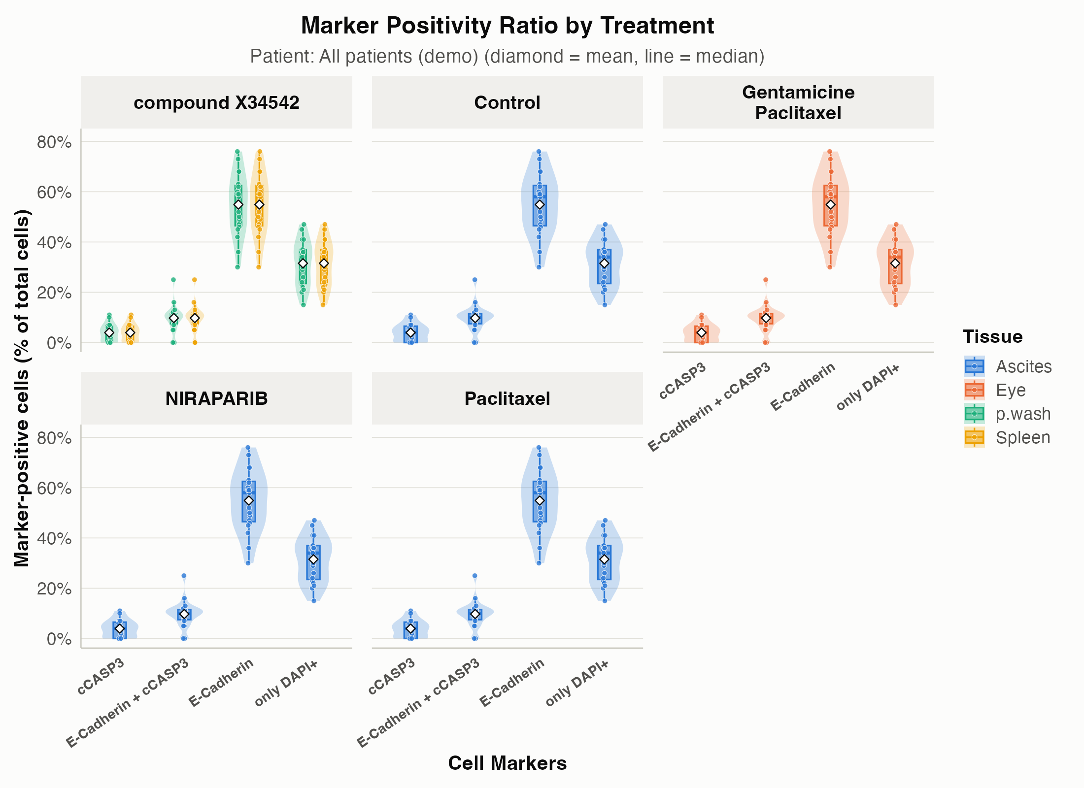
This function will change the wider format into longer format keeping all the metadata
plotting_ready_dataframe <- change_data_format_to_longer(counts_dataframe)Visualizing the results of the previous steps is essential to asses your experiment.
get_QC_plots(plotting_ready_dataframe, save_plots = TRUE, isolate_a_specific_patient = "B39")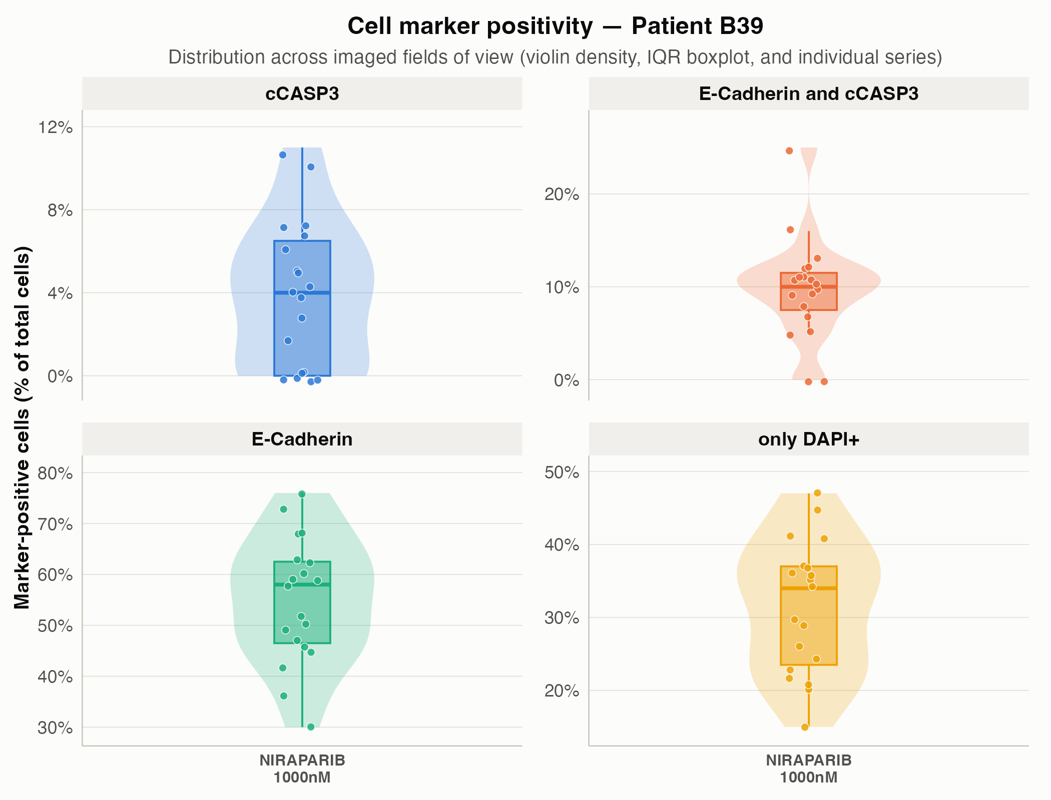
Let’s run drugsens with your data. drugsens
is not very strict about the capitalization of the file name but is very
strict on the position of the parameters. This to avoid potential
parsing problems. Here how the labeled data should look like in your
QuPath generated file. Here below is shown a the first row from the file
A8759_drug1..conc2.csv contained as example in
system.file("extdata/to_merge/", package = "drugsens")
A8759_p.wash_2020.11.10_DOC2001.10.05_compoundX34542_10000_uM_EpCAM_Ecad_cCasp3_(series 01).tifThat follows the structure suggested in the QuPath script
"<USER_DEFINED_PATH>/<PID>_<TISSUE>_<YYYY-MM-DD>_<SAMPLE_DOC>_<TREATMENT_INITIALS>_<CONCENTRATION>_<CONCENTRATION_UNITS>_<REPLICA_OR_NOT>_<TUMOR_MARKER>_<APOPTOTIC_MARKER>.csv"Warning: Follow the field order above so
string_parsing()assigns every token to the right column (YYYY-MM-DDdates,CamelCasefor two-drug combinations such asCarboplatinPaclitaxel_100_uM_10_nM, and.as a placeholder for missing tokens). See the QuPath & Metadata tutorial for worked examples.
These lines sets stage for drugsens to find the
directory path where the microscopy image data are located.
defined_path is a predefined variable that should contain
the base path. This makes it easier to access and manage the files
during processing. It is convenient also to define the
desired_file_extensions_of_the_files, usually
csv is a good start.
defined_path <- "<USER_DEFINED_PATH>"
desired_file_extensions <- "csv"
You can then
bind_data <- data_binding(path_to_the_projects_folder = defined_path,
files_extension_to_look_for = desired_file_extensions, recursive_search = FALSE)
Note: Set
recursive_search = FALSEindata_binding()if your target directory contains subfolders from other projects or staining panels.
Each file is read, and additional metadata is extracted. This will return a dataframe of all the csv files within the folder merged with some additional parsing, the metadata is parsed from the file name will be retrieved and appended to the data. Metadata such as:
DOC = The date when the biological sample was
collected.Tissue = Indicates the type of tissue from which the
sample was derived. This could be a specific organ or cell typeImage_number = Represents the order or sequence number
of the image in a stack of imagesTreatment = The name or type of drug treatment applied
to the sampleConcentration = The amount of the drug treatment
applied (concentration), quantitatively described.ConcentrationUnits = The units in which the drug
concentration is measured, such as micromolar (uM) or nanomolar
(nM)ReplicaOrNot = Indicates whether the sample is a
replica or repeat of a previous experimentName = The standardized name of the cell markers as
defined in the config_drugsens.txt file. This ensures
consistency and accuracy in identifying and referring to specific cell
markers.plots <- get_QC_plots_parsed_merged_data(bind_data,
fill_color_variable = "Treatment_complete", save_plots = TRUE)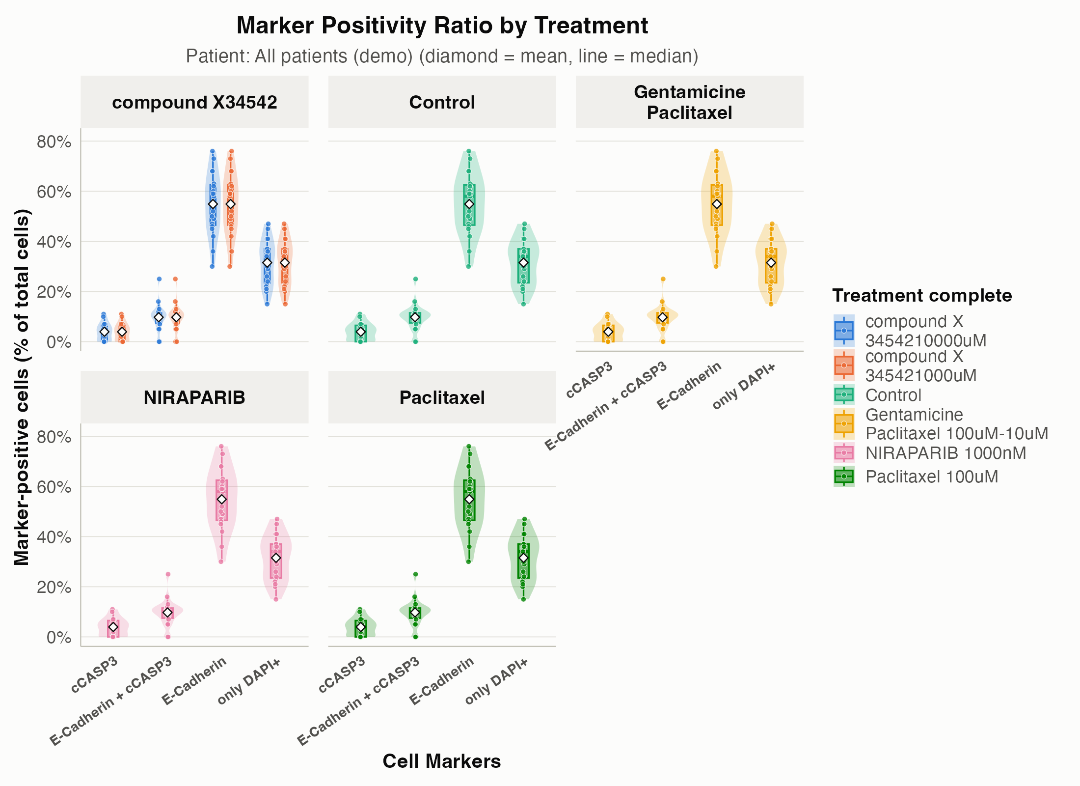
This plot shows the ratio of expressed markers across the various
conditions; other variables (for example Tissue or
Treatment_complete) can also be used. When
save_plots = TRUE and
saving_plots_folder = NULL, files are saved in
file.path(tempdir(), "drugsens_plots") with subfolders for
each PID present in the dataset.
.data: The main dataset, expected to be a dataframe
that has been preprocessed and formatted into a long format.list_of_columns_to_plot: Specifies which columns in the
data should be visualized. Defaults to all numeric columns if not
provided.save_plots: A boolean flag indicating whether the plots
should be saved as files.saving_plots_folder: The directory where plot files
will be saved, defaulting to
file.path(tempdir(), "drugsens_plots") when
NULL.fill_color_variable: Specifies a variable in the data
to use for color-coding the plots, enhancing the visual distinction
between different data groups.PID_column_name, isolate_specific_drug,
isolate_specific_patient: Parameters allowing for the isolation of data
based on patient ID or specific treatment, facilitating targeted
analysis.drug_column_name: Defines the column that indicates the
treatment or drug, with “Treatment” as the default.save_list_of_plots,
save_plots_in_patient_specific_subfolders: Flags
controlling the saving behavior of the plots, including the option to
save in patient-specific subfolders for organized file management.p_height, p_width: Parameters to customize
the height and width of the generated plots, ensuring they fit the
desired visualization scale.make_count_dataframe(), is designed for processing
microscopy data stored in a dataframe. It counts occurrences of
different markers present in the dataset and computes additional
metadata based on unique identifiers within each row.
cell_markers_counts_data <- make_count_dataframe(bind_data).data: The input dataframe containing microscopy
data.unique_name_row_identifier: The name of the column in
.data that contains unique identifiers for each row (default is
“filter_image”).name_of_the_markers_column: The name of the column in
.data that contains the names of the markers (default is “Name”).Note:
make_count_dataframe()acceptsbind_datadirectly with default settings. If you renamed the image identifier or marker column, pass your custom column names viaunique_name_row_identifierandname_of_the_markers_column.
The data output will be a dataframe, with all the metadata coming from the previous preprocessing. At this point, you can you the data already, but you can additionally change the format from wider to longer. This is useful especially for plotting and more fine analysis.
change_data_format_to_longer, transforms count data from
a wide format to a longer format, making it more suitable for certain
types of analysis or visualization. - .data: The input
dataframe containing count data in a wide format, typically generated
from microscopy data processing. - pattern_column_markers:
A pattern used to identify columns related to marker ratios (defaults to
“_ratio_of_total_cells”). - unique_name_row_identifier: The
name of the column in .data that contains unique identifiers for each
image (defaults to “filter_image”). - additional_columns: A
logical value indicating whether to include additional metadata columns
in the longer format dataframe. It defaults to TRUE.
plotting_format <- change_data_format_to_longer(cell_markers_counts_data)Note:
change_data_format_to_longer()acceptscell_markers_counts_datadirectly. If you customized the marker ratio suffix or image identifier column, specifypattern_column_markers,unique_name_row_identifier, oradditional_columns.
This will return a dataframe that can be easily used for plotting and additional analyses.
get_QC_plots, is designed for generating Quality Control (QC) plots from preprocessed microscopy data. It visualizes cell marker ratios across different treatments for each patient or a specific patient, aiding in the immediate assessment of data quality and trends. Input Parameters:
get_QC_plots(plotting_format, isolate_a_specific_patient = "A8759", save_plots = T)More parameters can be specified to personalize the plot(s).
.data: The preprocessed and merged dataframe, expected
to be in a long format, typically obtained after processing through
make_count_dataframe() and change_data_format_to_longer().patient_column_name: Specifies the column in .data that
contains patient identifiers (defaults to “PID”).colors: A vector of colors for the plots. Defaults to
unname(drugsens_palette) (an 8-color CVD-safe
palette).save_plots: A Boolean flag indicating whether to save
the generated plots. If TRUE, plots are saved in the specified
directory.folder_name: The directory where plots will be saved if
save_plots = TRUE. Defaults to
file.path(tempdir(), "figures") when
NULL.isolate_a_specific_patient: If specified, QC plots will
be generated for this patient only. Defaults to NULL, meaning plots will
be generated for all patients.x_plot_var: The variable to be used on the x-axis,
typically indicating different treatments. Defaults to
“Treatment_complete”.Once you have plotting-ready data,
normalize_to_control() expresses every marker value as a
percentage of the mean control (vehicle/untreated) value, per patient.
This is the standard first step before building dose response
curves.
normalized <- normalize_to_control(plotting_format)control_treatment_name: The value in
treatment_column_name that identifies control/vehicle
wells. Defaults to “Control”.group_by_columns: Columns that define a comparable
batch; the control mean is computed within each combination of these
columns. Defaults to “PID”.plot_normalization_before_after() then shows the raw
ratio next to the normalized percent-of-control value, one pair of
panels per marker, so you can see at a glance what normalization did to
the data:
plot_normalization_before_after(normalized)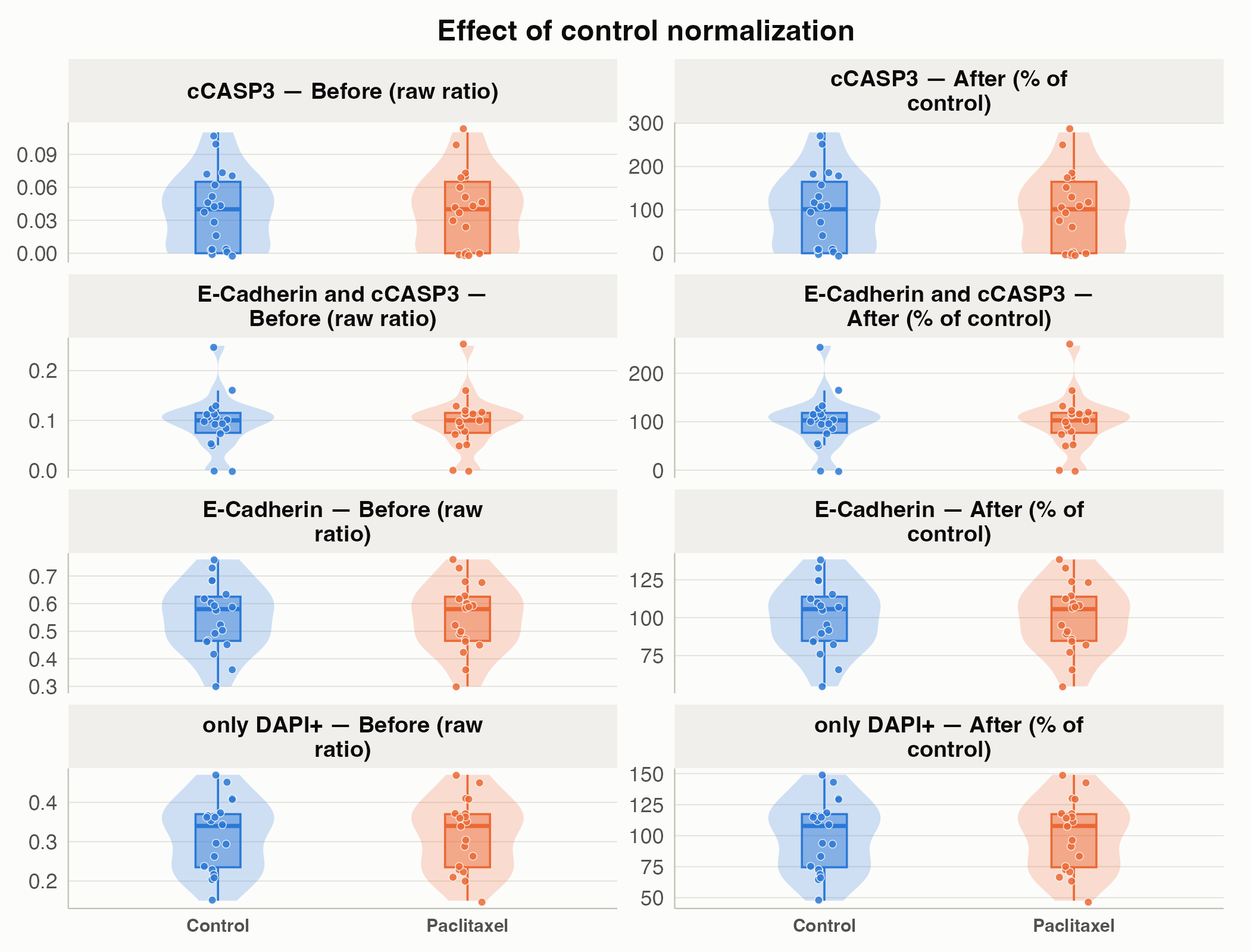
From there, plot_dose_response(),
plot_dose_response_heatmap(),
plot_treatment_summary(), and
plot_patient_heatmap() all build on the normalized data to
give dose-response curves, treatment x concentration and patient x
treatment overviews, and a ranked summary of the whole drug panel. See
the function
reference for details on each.
We welcome contributions from the community! Here are some ways you can contribute:
To get started with development, follow these setup instructions:
This project uses renv for R package management to
ensure reproducibility. To set up your development environment:
renv::restore() to install the required R
packages.Renv will automatically activate and install the necessary packages
as specified in the renv.lock file.
If you encounter any bugs or have suggestions for improvements, please file an issue on GitHub Issues: https://github.com/flalom/drugsens/issues. Be sure to include as much information as possible to help us understand and address the issue. BugReports: https://github.com/flalom/drugsens/issues