


Country names never line up across data sources. "US",
"U.S.", "United States",
"United States of America" and "America" are
the same country, but a naïve left_join() treats them as
five. countryatlas kills that pain by making
ISO codes the universal join key and handing you a
single, ready-to-map tibble that already stitches together three
otherwise disjoint worlds:
ggplot2::map_data("world") (or Natural
Earth sf) — where countries are,The happy path is one call: world_data(2020). Everything
else is opt-in.
as_ggsql_source(),
world_query(),
interactive_map(engine = "ggsql").globe_map()), small multiples (facet_map()),
and 8 more projections (Winkel tripel, orthographic, Gall–Peters,
…).locate_country() (point-in-polygon).repair_country_names()
auto-fixes typos; country_join_all() reduce-joins many
tables at once.growth_rate(),
index_to(), share_of_world().country_borders() /
neighbors() (who borders whom),
distance_between() (great-circle distance, no
sf needed) and morans_i() (spatial
autocorrelation on the package’s own adjacency — no
spdep).dissolve_country() + the historical_codes
crosswalk resolve the USSR / Yugoslavia / Czechoslovakia to successor
states; check_country_match() now flags them (countrycode
silently maps "USSR" to Russia — caught).gini(),
theil() (population-weighted, between/within
decomposition), beta_convergence(),
sigma_convergence(), correlate_indicators(),
lag_by_country() / diff_by_country().dorling_map() and
spike_map(): two more honest displays for
totals.convert_country(to = "name_fr" / "name_es" / …).# install.packages("devtools")
devtools::install_github("PursuitOfDataScience/countryatlas")The base install is light. Heavy spatial extras (sf,
rnaturalearth, cartogram,
biscale, gganimate, leaflet, …)
live in Suggests and are only needed for the features that
use them.
| Feature / verb | Optional packages required |
|---|---|
world_map() polygon backend, spike_map(),
flow_map(), bubble_map() |
maps |
sf geometry: world_map(sf),
world_geometry(sf), locate_country(),
country_borders(), neighbors(),
morans_i() |
sf, rnaturalearth,
rnaturalearthdata |
globe_map(backend = "polygon") |
maps, mapproj |
spin_globe() (animated GIF) |
its backend’s packages, plus gifski or
magick |
bivariate_map() |
biscale, sf |
cartogram_map(), dorling_map() |
cartogram, sf |
animate_world() (animated GIF) |
gganimate (+ gifski or
magick) |
interactive_map(engine = "plotly") |
plotly |
interactive_map(engine = "ggiraph") |
ggiraph |
interactive_map(engine = "leaflet") |
leaflet, sf |
interactive_map(engine = "ggsql") |
ggsql (>= 0.4.1), duckdb,
DBI, sf |
as_ggsql_source() |
duckdb + DBI, or nanoarrow
for format = "arrow" |
simplify_geometry() |
sf; rmapshaper for the better
simplifier |
repair_country_names() /
check_country_match() with stringdist |
stringdist |
library(countryatlas)
library(ggplot2)
library(dplyr)data_2020 <- world_data(2020)
data_2020
#> # A tibble: 99,338 × 12
#> long lat group order subregion iso3c iso2c country continent region income
#> <dbl> <dbl> <dbl> <int> <chr> <chr> <chr> <chr> <chr> <chr> <fct>
#> 1 -69.9 12.5 1 1 <NA> ABW AW Aruba Americas Latin… High …
#> 2 -69.9 12.4 1 2 <NA> ABW AW Aruba Americas Latin… High …
#> 3 -69.9 12.4 1 3 <NA> ABW AW Aruba Americas Latin… High …
#> 4 -70.0 12.5 1 4 <NA> ABW AW Aruba Americas Latin… High …
#> 5 -70.1 12.5 1 5 <NA> ABW AW Aruba Americas Latin… High …
#> 6 -70.1 12.6 1 6 <NA> ABW AW Aruba Americas Latin… High …
#> 7 -70.0 12.6 1 7 <NA> ABW AW Aruba Americas Latin… High …
#> 8 -70.0 12.6 1 8 <NA> ABW AW Aruba Americas Latin… High …
#> 9 -69.9 12.5 1 9 <NA> ABW AW Aruba Americas Latin… High …
#> 10 -69.9 12.5 1 10 <NA> ABW AW Aruba Americas Latin… High …
#> # ℹ 99,328 more rows
#> # ℹ 1 more variable: gdp_per_capita <dbl>world_data() returns the map geometry, the requested
World Bank indicator(s), income and continent — already keyed on
iso3c/iso2c. Draw a choropleth with the
built-in world_map() helper (no more hand-rolled
geom_polygon() boilerplate):
world_map(data_2020, gdp_per_capita, style = "quantile",
          title = "GDP per capita, 2020")
world_map(data_2020, income, style = "categorical")
Pass one or many WDI codes with friendly names, or a year range to get a panel:
country_data(2020, c(life_exp = "SP.DYN.LE00.IN", co2 = "EN.GHG.CO2.PC.CE.AR5")) |>
  head()
#> # A tibble: 6 × 8
#>   iso3c iso2c country        continent region           income life_exp      co2
#>   <chr> <chr> <chr>          <chr>     <chr>            <fct>     <dbl>    <dbl>
#> 1 AFG   AF    Afghanistan    Asia      Middle East, No… Low i…     61.5  0.311
#> 2 ALB   AL    Albania        Europe    Europe & Centra… Upper…     77.8  1.81
#> 3 DZA   DZ    Algeria        Africa    Middle East, No… Upper…     73.3  3.90
#> 4 ASM   AS    American Samoa Oceania   East Asia & Pac… High …     72.7  0.00201
#> 5 AND   AD    Andorra        Europe    Europe & Centra… High …     79.4 NA
#> 6 AGO   AO    Angola         Africa    Sub-Saharan Afr… Lower…     63.1  0.614
Use the bundled common_indicators catalogue so you never
memorise a code, or search the full World Bank catalogue offline with
wdi_search():
head(common_indicators)
#> # A tibble: 6 × 3
#>   name                   code           description
#>   <chr>                  <chr>          <chr>
#> 1 population             SP.POP.TOTL    Population, total
#> 2 gdp                    NY.GDP.MKTP.CD GDP (current US$)
#> 3 gdp_constant           NY.GDP.MKTP.KD GDP (constant 2015 US$)
#> 4 gdp_per_capita         NY.GDP.PCAP.KD GDP per capita (constant 2015 US$)
#> 5 gdp_per_capita_current NY.GDP.PCAP.CD GDP per capita (current US$)
#> 6 gni_per_capita         NY.GNP.PCAP.CD GNI per capita (current US$)
wdi_search("renewable energy") |> head(3)
#> # A tibble: 3 × 2
#>   indicator                    name
#>   <chr>                        <chr>
#> 1 2.1_SHARE.TOTAL.RE.IN.TFEC   Renewable energy consumption(% in TFEC)
#> 2 3.1_RE.CONSUMPTION           Renewable energy consumption (TJ)
#> 3 4.1.2_REN.ELECTRICITY.OUTPUT Renewable energy electricity output (GWh)This is the headline use case. You have a frame keyed on messy
country names — join_world() standardises it and attaches
geometry in one call:
my_data <- data.frame(
  nation = c("U.S.", "S. Korea", "Czechia", "Kosovo", "Cote d'Ivoire"),
  score  = c(10, 8, 6, 4, 7)
)

my_data |>
  join_world(nation, warn = FALSE) |>
  world_map(score, title = "My data, joined on the ISO spine")
Or reconcile two messy tables directly —
"Czech Republic" vs "Czechia",
"South Korea" vs "Korea, Rep." just work:
a <- data.frame(country = c("Czechia", "South Korea"), gdp = c(1, 2))
b <- data.frame(nation  = c("Czech Republic", "Korea, Rep."), pop = c(10, 51))
country_join(a, b, country, nation)
#> # A tibble: 2 × 5
#>   country       gdp iso3c nation           pop
#>   <chr>       <dbl> <chr> <chr>          <dbl>
#> 1 Czechia         1 CZE   Czech Republic    10
#> 2 South Korea 2 KOR Korea, Rep. 51check_country_match(c("USA", "Cote d'Ivoire", "Yugoslavia", "Wakanda"))
#> # A tibble: 4 × 5
#> input iso3c matched historical suggestion
#> <chr> <chr> <lgl> <lgl> <chr>
#> 1 USA USA TRUE FALSE <NA>
#> 2 Cote d'Ivoire CIV TRUE FALSE <NA>
#> 3 Yugoslavia <NA> FALSE TRUE Yugoslavia
#> 4 Wakanda <NA> FALSE FALSE Canadaconvert_country(c("Japan", "Brazil", "Germany"), to = "flag")
#> [1] "🇯🇵" "🇧🇷" "🇩🇪"
convert_country(c("Japan", "Brazil", "Germany"), to = "currency")
#> [1] "JPY" "BRL" "EUR"
in_group(c("France", "United States", "Japan"), "EU")
#> [1] TRUE FALSE FALSEBeyond the choropleth: proportional-symbol
(bubble_map()), spikes (spike_map()),
bivariate (bivariate_map()), area-honest cartograms
(cartogram_map(), including a first-class
dorling_map()), equal-area tile grids
(tile_map()), great-circle flows (flow_map()),
an orthographic globe (globe_map()), small multiples
(facet_map()), animation (animate_world()) and
interactivity (interactive_map()).
The world as a globe, not a rectangle — with the
"polygon" backend (only maps +
mapproj, no sf) you can draw it and even
spin it:
globe_map(world_snapshot$countries, continent, backend = "polygon",
          style = "categorical", lon = 10, lat = 20)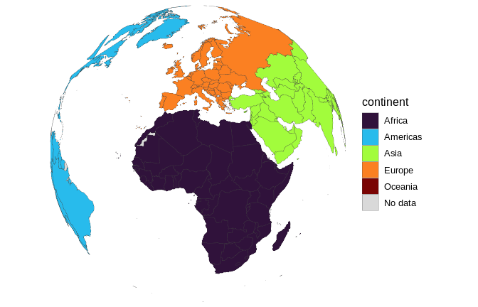
# assemble a rotating GIF (one full turn; needs gifski or magick)
spin_globe(world_snapshot$countries, continent, backend = "polygon",
           style = "categorical")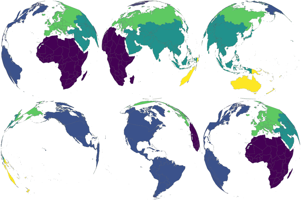
bubble_map(world_snapshot$countries, population)
ggsql draws plots in the
database (DuckDB) and returns a Vega-Lite widget — no ggplot2 or
sf runtime needed. countryatlas does the part ggsql’s
static world can’t (ISO reconciliation, overrides, the WDI join); ggsql
does the part countryatlas doesn’t (push-down + web-ready output).
world_query() emits the spatial query (no
dependencies):
world_query(gdp_per_capita, palette = "magma", transform = "log10",
            title = "GDP per capita")
#> VISUALISE gdp_per_capita AS fill
#> FROM countryatlas_world
#> DRAW spatial
#> PROJECT TO equal_earth
#> SCALE fill TO magma VIA log10
#> LABEL title => 'GDP per capita'
…and as_ggsql_source() /
interactive_map(engine = "ggsql") register your curated
table and render it in the database. See the countryatlas and
ggsql vignette.
Get point data onto the spine, repair messy names, reduce-join many
tables, and run panel analysis — all keyed on iso3c:
# normalise a total by population, so the map isn't just a population map
# (omit `pop` and SP.POP.TOTL is fetched for the relevant countries/years)
per_capita(data.frame(iso3c = c("USA", "CHN"), co2 = c(4.7e6, 1.1e7),
                      pop = c(331e6, 1412e6)), co2, pop)
#> # A tibble: 2 × 4
#>   iso3c      co2        pop co2_per_capita
#>   <chr>    <dbl>      <dbl>          <dbl>
#> 1 USA    4700000  331000000        0.0142
#> 2 CHN   11000000 1412000000        0.00779

# each country's share of a world total (within year, for a panel)
share_of_world(data.frame(iso3c = c("USA", "CHN", "IND"), co2 = c(5, 15, 3)), co2)
#> # A tibble: 3 × 3
#>   iso3c   co2 co2_share
#>   <chr> <dbl>     <dbl>
#> 1 USA       5     0.217
#> 2 CHN      15     0.652
#> 3 IND       3     0.130

# reduce-join several messy tables on the ISO spine at once
t1 <- data.frame(country = c("Czechia", "South Korea"), gdp = c(1, 2))
t2 <- data.frame(country = c("Czech Republic", "Korea, Rep."), pop = c(10, 51))
t3 <- data.frame(country = c("Czechia", "Korea"), area = c(79, 100))
country_join_all(list(t1, t2, t3), by = "country")
#> # A tibble: 2 × 7
#>   country.x     gdp iso3c country.y        pop country  area
#>   <chr>       <dbl> <chr> <chr>          <dbl> <chr>   <dbl>
#> 1 Czechia         1 CZE   Czech Republic    10 Czechia    79
#> 2 South Korea     2 KOR   Korea, Rep.       51 Korea     100

# great-circle distance between two countries' centroids (no sf needed)
distance_between("France", "Germany")
#> [1] 802.3524Dissolved entities poison country joins twice over: most are silently
dropped, and some are silently mismatched — countrycode
resolves "USSR" to Russia alone, so Soviet-era totals
quietly become Russian totals. check_country_match() flags
both cases, and dissolve_country() resolves them to
successor states (one-to-many, dated) via the curated
historical_codes crosswalk:
check_country_match(c("USSR", "Yugoslavia", "France"))
#> # A tibble: 3 × 5
#>   input      iso3c matched historical suggestion
#>   <chr>      <chr> <lgl>   <lgl>      <chr>
#> 1 USSR       RUS   TRUE    TRUE       <NA>
#> 2 Yugoslavia <NA>  FALSE   TRUE       Yugoslavia
#> 3 France     FRA   TRUE    FALSE      <NA>
dissolve_country("Czechoslovakia")
#> # A tibble: 2 × 5
#>   input          historical     dissolved iso3c country
#>   <chr>          <chr>              <int> <chr> <chr>
#> 1 Czechoslovakia Czechoslovakia      1993 CZE   Czechia
#> 2 Czechoslovakia Czechoslovakia 1993 SVK SlovakiaWorld inequality between people, not country units — and how much of it sits between continents vs within them:
snap <- world_snapshot$countries
gini(snap$gdp_per_capita, weights = snap$population)
#> [1] 0.6094909
theil(snap$gdp_per_capita, weights = snap$population, groups = snap$continent)
#> # A tibble: 3 × 3
#>   component value share
#>   <chr>     <dbl> <dbl>
#> 1 total     0.678 1
#> 2 between   0.310 0.458
#> 3 within    0.368 0.542
beta_convergence() / sigma_convergence()
test whether poor countries are catching up;
correlate_indicators() screens indicator pairs
(pairwise-complete, with n reported); and
morans_i() measures spatial autocorrelation on the
package’s own border adjacency — no spdep required.
repair_country_names() auto-fixes typos to the closest
known country, locate_country(lon, lat) tags coordinates
with the country that contains them, neighbors() /
country_borders() answer “who shares a border with whom”,
growth_rate() / index_to() /
complete_years() add panel metrics and fill panel gaps, and
country_codes() exposes the whole countrycode crosswalk as
a tidy, pipeable lookup.
The bundled world_snapshot (a curated indicator set for
one recent year, plus metadata) means examples, tests and vignettes all
run without the World Bank API.
See the vignettes — Getting started, Joining your own data, Modern maps with sf & projections, Beyond the choropleth, and countryatlas and ggsql — and the reference site.