


The {choicedata} package simplifies working with choice
data in R.
Install the released version from CRAN:
install.packages("choicedata")The package breaks choice-data modeling into a series of objects. Each object contains the information needed for the next step.
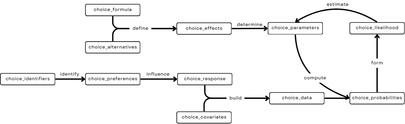
choice_formula:
the choice model formula.
choice_alternatives:
the set of choice alternatives.
choice_effects:
the choice effects, defined by choice_alternatives and
choice_formula.
choice_parameters:
the model parameters, determined by choice_effects and
estimated via choice_likelihood.
choice_identifiers:
the identifiers for deciders and choice occasions.
choice_preferences:
the choice preferences of the deciders, identified by
choice_identifiers.
choice_responses:
the choice responses, influenced by
choice_preferences.
choice_covariates:
the choice covariates.
choice_data:
the choice data, built by choice_covariates and
choice_responses.
choice_probabilities:
the choice probabilities, computed from choice_data and
choice_parameters.
choice_likelihood:
the likelihood of the choice model, formed by
choice_probabilities.
The objects are designed to be modular and can be combined in various ways to create a range of modeling workflows.
The TravelMode data set of the AER
package (Kleiber and Zeileis 2008)
contains the revealed preferences of 210 travelers choosing between air,
train, bus, and car:
library("choicedata")
data("TravelMode", package = "AER")
TravelMode$choice <- TravelMode$choice == "yes"
head(TravelMode)
#>   individual  mode choice wait vcost travel gcost income size
#> 1          1   air  FALSE   69    59    100    70     35    1
#> 2          1 train  FALSE   34    31    372    71     35    1
#> 3          1   bus  FALSE   35    25    417    70     35    1
#> 4          1   car   TRUE    0    10    180    30     35    1
#> 5          2   air  FALSE   64    58     68    68     30    2
#> 6          2 train  FALSE   44    31    354    84     30    2
We can transform the data from long (one row per choice alternative) to wide format (one row per choice occasion):
long_to_wide(
  data_frame = TravelMode,
  column_alternative = "mode",
  column_decider = "individual"
)
#> # A tibble: 210 × 20
#>    individual income  size wait_air wait_train wait_bus wait_car vcost_air
#>    <fct>       <int> <int>    <int>      <int>    <int>    <int>     <int>
#>  1 1              35     1       69         34       35        0        59
#>  2 2              30     2       64         44       53        0        58
#>  3 3              40     1       69         34       35        0       115
#>  4 4              70     3       64         44       53        0        49
#>  5 5              45     2       64         44       53        0        60
#>  6 6              20     1       69         40       35        0        59
#>  7 7              45     1       45         34       35        0       148
#>  8 8              12     1       69         34       35        0       121
#>  9 9              40     1       69         34       35        0        59
#> 10 10             70     2       69         34       35        0        58
#> # ℹ 200 more rows
#> # ℹ 12 more variables: vcost_train <int>, vcost_bus <int>, vcost_car <int>,
#> #   travel_air <int>, travel_train <int>, travel_bus <int>, travel_car <int>,
#> #   gcost_air <int>, gcost_train <int>, gcost_bus <int>, gcost_car <int>,
#> #   choice <fct>
We can construct model design matrices:
mode_data <- choice_data(
  data_frame = TravelMode,
  format = "long",
  column_choice = "choice",
  column_decider = "individual",
  column_alternative = "mode",
  column_ac_covariates = c("income", "size"),
  column_as_covariates = c("wait", "vcost", "travel", "gcost")
)

mode_effects <- choice_effects(
  choice_formula = choice_formula(
    formula = choice ~ vcost | income | wait,
    error_term = "probit"
  ),
  choice_alternatives = choice_alternatives(
    alternatives = levels(TravelMode$mode)
  ),
  choice_data = mode_data
)

mode_design <- design_matrices(mode_data, mode_effects)
mode_design[[1]] |> round()
#>       vcost income_bus income_car income_train ASC_bus ASC_car ASC_train
#> air      59          0          0            0       0       0         0
#> bus      25         35          0            0       1       0         0
#> car      10          0         35            0       0       1         0
#> train    31          0          0           35       0       0         1
#>       wait_air wait_bus wait_car wait_train
#> air         69        0        0          0
#> bus          0       35        0          0
#> car          0        0        0          0
#> train 0 0 0 34generate_choice_data() makes it straightforward to
simulate choice data. The example below simulates 200 ranking tasks with
three alternatives and recovers the data-generating parameters by
optimizing the likelihood:
library("choicedata")

set.seed(1)

sim_effects <- choice_effects(
  choice_formula = choice_formula(
    formula = choice ~ x | y + 0 | z,
    error_term = "logit"
  ),
  choice_alternatives = choice_alternatives(
    J = 3,
    alternatives = c("A", "B", "C")
  )
)

sim_parameters <- generate_choice_parameters(sim_effects)

(sim_data <- generate_choice_data(
  choice_effects = sim_effects,
  choice_identifiers = generate_choice_identifiers(N = 200),
  choice_parameters = sim_parameters,
  choice_type = "ranked"
))
#> # A tibble: 200 × 13
#>    deciderID occasionID choice       y    x_A     x_B     x_C     z_A    z_B
#>  * <chr>     <chr>      <chr>    <dbl>  <dbl>   <dbl>   <dbl>   <dbl>  <dbl>
#>  1 1         1          B      -0.621   0.487  0.738   0.576  -0.305   1.51
#>  2 2         1          A       0.594  -2.21   1.12   -0.0449 -0.0162  0.944
#>  3 3         1          C      -0.156   0.919  0.782   0.0746 -1.99    0.620
#>  4 4         1          A      -0.0538 -1.47  -0.478   0.418   1.36   -0.103
#>  5 5         1          B      -0.165  -1.38  -0.415  -0.394  -0.0593  1.10
#>  6 6         1          A       0.769  -0.253  0.697   0.557  -0.689  -0.707
#>  7 7         1          B       1.43   -0.112  0.881   0.398  -0.612   0.341
#>  8 8         1          B      -0.0392  1.98  -0.367  -1.04    0.570  -0.135
#>  9 9         1          A       0.153   0.690  0.0280 -0.743   0.189  -1.80
#> 10 10        1          C       0.291   2.17   0.476  -0.710   0.611  -0.934
#> # ℹ 190 more rows
#> # ℹ 4 more variables: z_C <dbl>, choice_A <int>, choice_B <int>, choice_C <int>

sim_likelihood <- choice_likelihood(
  choice_data = sim_data,
  choice_effects = sim_effects
)

true_vector <- switch_parameter_space(
  choice_parameters = sim_parameters,
  choice_effects = sim_effects
)

fit <- stats::optim(
  par = stats::rnorm(length(true_vector)),
  fn = function(par) {
    compute_choice_likelihood(
      choice_parameters = par,
      choice_likelihood = sim_likelihood,
      logarithm = TRUE,
      negative = TRUE
    )
  }
)

estimated_parameters <- switch_parameter_space(
  choice_parameters = fit$par,
  choice_effects = sim_effects
)

data.frame(dgp = true_vector, estimated = fit$par) |> round(2)
#>          dgp estimated
#> beta_1 -1.98     -2.36
#> beta_2  0.58      0.53
#> beta_3 -2.64     -2.83
#> beta_4  5.04      5.64
#> beta_5  1.04      1.18
#> beta_6 -2.59 -3.03{Rprobit} (Bauer et
al. 2023) provides maximum approximated composite marginal
likelihood estimation for efficient probit choice modeling.
{RprobitB} (Oelschläger
and Bauer 2025) provides Bayesian tools for estimating probit
models.
You have a question, found a bug, or want to contribute? Please file an issue on GitHub.